Socioeconomic Analysis of Crime in Vancouver  

Preparing for Analysis

​

After obtaining the census data, the first step was to link the attribute data to the Vancouver dissemination area geography file through a joining of the table to the file. Following that, combining the crime data with the census data using spatial joins is necessary, which would summarize the number of crime events within the respective spatial units (DA).

​

Regression and Spatial Autocorrelation

​

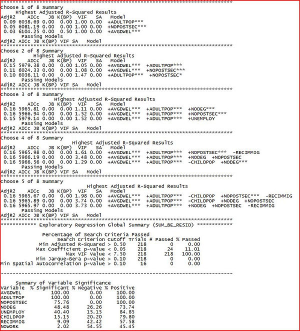
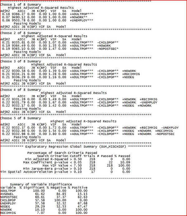
A simple regression and spatial autocorrelation is then done afterwards where an Ordinary Least Squares model is conducted in order to determine how  far/close residuals are.  Three OLS models were created to reflect each of the categories of crime as dependent variables: Break and enters, Mischief, and Auto theft. The explanatory variables were taken from the socioeconomic attribute data that was entered before: House value, Population of adults (18+), Population of children (0-18), Population with postsecondary degree, Unemployed population, and recent immigrant population. Before starting the OLS, in order to determine the most important explanatory variables to use for each respective dependent crime variables within the OLS model, an Exploratory Regression Analysis needs to be carried out. After the most important dependent variables are determined with having the highest AdjR2 values as well as the lowest AICc, the OLS model can be utilized. The OLS regression model is expressing the relation between the socioeconomic factors (x) and crime data (y) in that area. In effect, the socioeconomic factors in a DA are used to predict the number of crime occurring in that area. The (aspatial) regression model produces an equation (a linear model between socioeconomic factors and crime data) that summarizes the relation for the entire study region (all of the City of Vancouver).

​

​

​

​

​

​

​

​

​

​

​

​

​

​

​

​

​

​

​

​

​

​

​

​

​

​

​

​

​

​

​

​

​

 

 

 

 

Chosen explanatory variables for Break and Enter: House Value, Population of Adults, No Post-secondary degree

​

​

​

​

​

​

​

 

 

 

 

 

 

 

 

 

 

 

 

 

 

 

 

 

 

 

 

 

 

 

 

 

 

Chosen explanatory variables for Mischief: Population of Adults, Population of Children and Population of Unemployment 

 

 

 

 

 

 

 

 

 

 

 

 

 

 

 

 

 

 

 

 

 

 

 

 

 

 

 

 

 

 

 

 

Chosen explanatory variables for Auto Theft: House Value, Population of Adults, Population of children,  No Post-secondary degree

 

Geographic Weighted Regression

A Geographic Weighted Regression is then conducted to explore the spatial nature of the relations. The GWR was performed with the dependent variables being the three categories of crime again as well as their respective explanatory variables determined by the previous exploratory regression analysis. The narrowed down most important explanatory variables included: house value, population of adults, population of children, population with post secondary degree, and unemployed population. With this, three GWR models were created with each of the three categories of crime with adaptive kernel type and BANDWIDTH_PARAMETER. Coefficient raster surfaces were manually made by converting DA polygons to rasters (cell size 50) and displayed in stretched symbology – Standard Deviation.

 

Grouping Analysis

​

A Grouping Analysis is also necessary to see if there are any areas within the city that exhibit similar patterns with respect to crime and socioeconomic factors. It illustrates what socioeconomic factors each crime “neighbourhood” has in common through mapping clusters. Five groups are used for both the census tracts and dissemination area. This Grouping Analysis took into account the exact same variables that mentioned and used for the GWR model as well.

 

Hotspot Analysis

​

Lastly a Hotspot Analysis was conducted using the original crime layer and the tool, Optimized Hotspot Analysis.